Principle Components Analysis

Many times in artificial intelligence we deal with large data sets of a large number of features or variables and there is not a clear way to visualize or interpret the relationships between these variables. Principle components analysis (PCA) is a technique for finding a basis set that may represent the data well under some circumstances. PCA finds a set of orthogonal basis vectors which are aligned in the directions of maximum variance, the so called principle components. PCA also ranks the components by importance (i.e. variance).

Principle components analysis assumes that the distributions of the random variables are characterizes by their mean and variance, exponential distributions such as the Gaussian distribution for example. PCA also makes the assumption that the direction of maximum variance is indeed the most “important”. This assumption implies that the data has a high signal-to-noise ratio; the variance added by any noise is small in comparison to the variance from the important dynamics of the system.

The principal components are calculated by finding the eigenvectors and eigenvalues of the covariance matrix. The covariance matrix is a square matrix which describes the covariance between random variables, where is the covariance between the th and th random variables. The random variables must be in mean deviation form, meaning that the mean has been subtracted so the distribution of the random variable has . The eigenvalues and eigenvectors are usually arranged such that is a diagonal matrix where the value of is the th eignenvalue , and is a matrix where the th column of is the th eigenvector. Note that the covariance matrix may have eigenvalues/eigenvectors, so and are matrices as well. At this point the eigenvectors can be ranked by importance by sorting the eigenvalues in . Since each eigenvector is associated with a particular eigenvalue, the columns of must be rearranged so the th column corresponds to the th eigenvalue.

If the goal is to reduce the dimensionality of the data set (the number of random variables), the principle components which are least important may be discarded. This leaves us with two matrices, where is the number of principal components to keep.

This matrix of eigenvectors represents a linear transform which orients the basis vectors in the directions of maximal variance, while maintaining orthogonality.

Read More

Basic Mathematical Structures and Operations

A mathematical structure is an association between one set of mathematical objects with another in order to give those objects additional meaning or power. Common mathematical objects include numbers, sets, relations, and functions.

An algebraic structure is defined by a collection of objects and the operations which are allowed to be applied to those objects. A structure may consist of a single set or multiple sets of mathematical objects (e.g. numbers). These sets are closed under a particular operation or operations, meaning that the result of the operation applied to any element of the set is also in the set. Axioms are conditions which the sets and operations must satisfy.

A simple but ubiquitous algebraic structure is the group. A group is a set and a single binary operation, usually denoted , which satisfy the axiom of associativity and contain and identity element and inverse elements. Associativity specifies that the order in which the operations are performed does not matter; that is . The identity element is a special element such that the operation applied to it and another element results in the other element; formally: . Each element of the set must have an inverse element that yields the identity element when the two are combined: . If the axiom of commutativity is added, the group is referred to as an Abelian group. Commutativity allows the operands to be reorganized: . If the requirement of inverse elements is removed from the group structure, the structure is called a monoid.

A group homomorphism is a function which preserves the relationships between the elements of the set, or the group structure. For groups and , is a homomorphism iff . If the map is invertible, i.e. it has an inverse such that , then is said to be an isomorphism. A group endomorphism is a homomorphism from a group onto itself, , while an invertible endomorphism is called a automorphism. A subgroup is a group within a larger group. For a subgroup of a group , and the identity element of is the identity element of .

A ring is an algebraic structure which adds another operations and a few axioms to the group structure. The operations and of a ring satisfy different axioms. The set and the addition operator must form an Abelian group as described above, while the set and the multiplication operator must form a monoid. In addition, the operators must satisfy the axiom of distribution, specifically the operator must be able to distribute over the operator, and . If forms a commutative monoid, that is, a monoid with commutativity, then the ring is said to be a commutative ring.

Similarly to a group, a ring may also have a ring homomorphism if satisfies and . Likewise, is an isomorphism if it has an inverse that satisfies the identity relation described for group isomorphism above. A ring is a subring of a ring if and contains the multiplicative identity from .

An algebraic structure is a field if it satisfies the axioms of a ring with a few addition axioms. Both operators of a field must satisfy commutativity, and the set must contain inverses under both operators, except that the field may not contain a multiplicative inverse for the additive identity element. Another way to describe a field is to say that the additive group is an Abelian group, and the multiplicative group without the additive identity is also an Abelian group. The inclusion of inverses for both operators lead to the intuitive notion of subtraction and division (except division by 0). An example of a well known field is the field of real numbers, .

A metric space is a mathematical structure , where is a binary function which defines the real-valued distance between two elements of the set . A distance is a non-negative quantity, and only equal to zero when the two element are equal. A distance should also satisfy the axiom of symmetry, and the triangle inequality . For example, the real-valued vector space equipped with the Euclidean distance metric yields the Euclidean metric space.

Read More

Smoothing

Like any captured signal, photographic images often suffer from the presence of noise. Noise produces variations in the captured signal that do not occur in the natural signal. That is, noise is introduced somewhere in the process of capturing the signal. It is usually viewed as an unwanted corruption of the signal, therefore the modeling and elimination of noise is an important part of signal processing. Noise can occur in a pattern, or be complex enough that it is modeled as a random phenomenon.

Noise can have many difference causes, and therefore manifest itself in many different ways. “Salt and pepper” noise is the term given to noise which causes the value of the signal at a particular point to be a random value. This has the effect of causing random spikes in the captured signal, regardless of the original signal, often called impulse noise. Quantizing the signal may cause noise as it is effectively assigning a particular value to a range of possible values, and therefore modifying the original values in a certain pattern. A common type of noise in amplified signals is Gaussian noise. The noise factor can be thought of as a random variable that follows a normal, or Gaussian, distribution. The noise factor can be added to the pixel value, called additive noise, or multiplied with the pixel value, multiplicative noise. When dealing with a potentially noisy signal it is often sufficient to take Gaussian noise into account to get acceptable results. Gaussian noise occurs in digital imagery as fluctuations in intensity values of the image. The noise is pixel-independent, meaning that the change in a pixel value is independent of the change in any other pixel value. It is also independent of the original intensity at each pixel. Since Gaussian noise is common and relatively simple it is commonly taken into consideration in generalized signal processing methods.

Noise can contribute noticeable artificial components to the image signal. Smoothing or blurring is a type of operation which attempts to eliminate the noise while preserving the structure of the image. The primary way this is accomplished is through the use of neighborhood filters. These are kernels, or matrices, which are convolved with the image in order to achieve some transformation, in this case smoothing.

One assumption we may be able to make is that the value of a pixel is relatively similar to the value of the neighboring pixels. Therefore, averaging together the pixel values in a small neighborhood should preserve the structure of the image while attenuating the effects of outlier values (the noise). This methods is called average smoothing, and is accomplished by convolving the image with a kernel in the following form, called a box filter:

Figure 1. Average Kernel

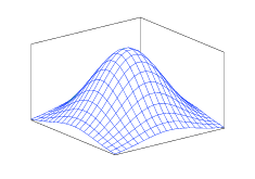
One issue with the box filter is that its rectangular window produces undesirable effects in the frequency domain. A Gaussian smoothing kernel provides a much better approximation of ideal smoothing. Intuitively the idea is that the neighboring pixels which are closer to the target pixel are weighted more heavily in the average than the pixels farther away. The weight coefficients follow a Gaussian distribution, producing a filter like the one shown in Figure 1. The Gaussian filter is desirable because of its gradual cutoff, producing a Gaussian distribution in the frequency domain as well which delivers smooth monotonically decreasing attenuation of higher frequencies. A Gaussian distribution has infinite width, however, the tails approach zero relatively rapidly so a few standard deviations of width are sufficient for accurate results.

gaussianeq

Figure 1. Gaussian Smoothing Kernel

Figure 2 shows a sample image and Figures 3, 4, & 5 show the effects of successively larger Gaussian smoothing kernels.


Figure 2. Sample Image


Figure 3. 3x3 Gaussian Blur
Figure 3. 3x3 Blur


Figure 4. 5x5 Gaussian Blur
Figure 4. 5x5 Blur


Figure 6. 10x10 Gaussian Blur
Figure 5. 10x10 BlurÂ

Read More

Convolution Transforms

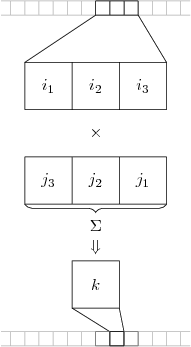
In a previous article we discussed the idea of the convolution sum as a way to filter a signal when we know the desired impulse response. Convolution is a widely used technique in image processing to apply transformations to the signal. Since images are two-dimensional functions the impulse response is also two-dimensional, a matrix commonly called a kernel. Kernels often apply transformations to small neighborhoods of pixels, but as they are swept across the entire image the image as a whole is transformed. Figure 1 shows a one-dimensional convolution operation, while Figure 2 shows a two-dimensional convolution.

Figure 1. One-Dimensional Convolution
Figure 2. Two-Dimensional Convolution

Here the values of represent the intensity values of the signal, while the values of represent the values of the kernel. Notice that the arrangement of the kernel values are reversed. Recall the formula for the convolution sum:

So the first value of the image neighborhood is multiplied with the last value of the kernel . The result of the convolution is the intensity value of the output signal at the center point of the neighborhood. To determine the output value at the convolution formula will take on the form .

In this way the kernel is “swept” across the image to determine the output value at each position. A problem arises when convolution is considered near the edges of the signal in a finite signal. For example, to determine the value of the convolution sum will require some values of which are not available (e.g., , etc) depending on the size of the kernel. What should be used in place of these values? There are several common approaches for dealing with this problem, called padding. The signal may be padded with enough zeros to satisfy the convolution sum, or the intensity values of the edge pixels may be replicated. Another approach is to mirror the pixel values about the edge, or to periodically repeat the pixel values. The resulting output signal will have a length of , where is the length of the input signal and is the length of the kernel. However, the only part of the output signal that is considered valid, that is does not contain padded values, the central part of the signal of length .

Cross-correlation is an operation similar to convolution, except it does not reverse the kernel when multiplying. Cross-correlation is often used to identify a the location of matching signals. A smaller signal is swept across a larger signal, when the signal is matched the values will be fully correlated resulting in maximal output.

Read More

Derivative Operations

One fundamental class of operations that can be performed to extract information from a signal is that of derivative operations. Just as derivatives are used in calculus to extract features of a curve or surface, the same ideas can be applied to a signal.

The first problem we have is that of taking the derivative of a discrete-time signal. Discrete-time signals are not continuous and are non-differentiable. However, we do know that if the Nyquist Rate was met when sampling, the continuous-time signal should be reconstructable from the discrete-time signal using the ideal sync. In order to reconstruct the continuous-time signal, the discrete-time signal is convolved with the ideal sync, . So if we want the derivative of the continuous time signal, we can start by taking the derivative of both sides of this equation.

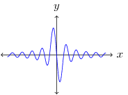
So the derivative of the continuous-time signal is equal to the convolution of the discrete-time signal with the derivative of the ideal sync. If instead the discrete-time signal is convolved with the sampled derivative ideal sync, this will result in a sampled derivative of the continuous-time signal, . The derivative of the ideal sync is shown in Figure 1. The major problem with this approach is that the derivative of the ideal sync is infinite and does not fall off rapidly.

Figure 1. Derivative of Ideal Sync

Designing filters to approximate the discrete-time derivative of the ideal sync are beyond the scope of this article, but several popular techniques will be described later.

If we want to apply derivative operations to an image we will have to extend this idea into 2-dimensional space. Using partial differentiation and a 2-dimensional ideal sync results in the following derivatives for :

The 2-dimensional ideal sync is said to be separable since it can be separated into its 1-dimensional components, . Again, these continuous-time derivatives of the ideal sync must be sampled. The horizontal and vertical derivative filters are denoted and , respectively.

The most basic approach to approximating is to use a version of the difference operator, that is, a sum of scaled differences of the samples, such as . This is accomplished by convolving with and amounts to an approximation of the derivative. Figure 2 shows an example of a row of pixel values from an image, while Figure 3 shows the derivative approximation of the pixel values and Figure 4 shows the second derivative. The locations where the intensity values change the most rapidly are represented by local peaks in the first derivative and zero-crossings in the second derivative. Note that taking the derivative extends the range of intensity values to allow negative values.

Figure 2. Original Intensity Values
Figure 3. Derivative
Figure 4. Second Derivative

If we think of the partial derivatives in each dimension as a component of a vector, this vector will represent the rate of change of the signal and the direction. This is called the gradient of the signal:

The gradient is a vector field where the direction of the vector at each point represents the direction of maximum change, while the magnitude of the vector represents the amount of change. As with other vectors, the magnitude can be calculated as , and the direction as . Given filters in the x and y directions, we can also construct a filter for an arbitrary direction, . Figure 4 shows a sample image and Figures 5 & 6 show the partial derivatives with respect to x and y respectively.

Figure 4. Sample Image
Figure 5. Sample Image
Figure 3. Horizontal Gradient
Figure 6. Horizontal Partial
Figure 4. Vertical Derivative
Figure 6. Vertical Partial

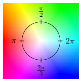
Figure 7 shows both the magnitude and the direction of the gradient of the sample image using the colormap in Figure 8. The partial derivative with respect to any direction, not just horizontal and vertical, can be calculated by multiplying a vector with the gradient, .

Figure 7. Gradient
Figure 7. Gradient
Figure 8. Colormap
Figure 8. Colormap

A useful tool when dealing with the second derivatives is the Hessian matrix which combines the derivatives into a matrix of the following form:

hessian

Where is the partial derivative of with respect to , i.e. the second derivative. To calculate the second derivative with respect to two vectors we can use the Hessian: .

Read More

Basic Image Processing

Basic image enhancement techniques allow us to manipulate an image to increase or decrease contrast and brightness. These techniques usually take the form of point-wise operations, meaning they act independently on each pixel of the image. An image is represented as a function mapping a pixel in 2-dimensional space to an intensity value, . The quantization method used when capturing the signal will determine the range of possible intensity values and their numeric representation, but will we assume that intensity values lie in the range [0,1]. Some types of images, such as color images, have more than one intensity spectrum or image plane, these are typically denoted as separate functions, such as , , and . Point-wise image operations can be performed using a transfer function that maps one set of intensity values to another set of intensity values, . This function can also be implemented as a lookup table, or LUT, when it is convenient.

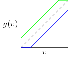
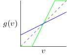
Linear functions are the most simple, although they typically involve undesirable clamping effects. To adjust the brightness of an image uniformly increase or decrease the intensities. The green line in Figure 1 represents an increase in brightness, while the blue line is a decrease. The dashed line is called the direct mapping, where the input of the function is directly mapped to the output, these are the original values. You can see that in order to keep intensity values within the [0, 1] range the higher end needs to be clamped when you increase brightness, and the lower end clamped when decreasing brightness. This has the effect of mapping multiple intensity values to the same value discarding information and creating and “washed out” look in the image.

Figure 1. Brightness Adjustment

Increasing or decreasing contrast can be accomplished by increasing or decreasing the slope of the transfer function. A slope of 0 turns the function into a horizontal line which maps all intensity values to the same value. A slope of creates a vertical line which maps the intensity values to just 2 values. This is called segmenting the image and the point at which the line crosses the -axis is called the threshold. All intensity values below the threshold are mapped to a certain intensity, while all the intensities values above the threshold are mapped to another. This creates a binary image with only two intensity values.

Figure 2. Contrast Adjustment

Linear operations can be combined to adjust brightness and contrast with the same transfer function. We can also decrease the amount of quantization using a step function. A step function with only two steps behaves the same as the thresholding technique described above creating a binary image.

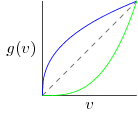
Non-linear functions are also useful for adjusting images. We may want to adjust the middle part of the transfer function but keep the endpoints at and . Gamma correction is a non-linear transfer function which affects the middle of the curve more than the endpoints. Note that the curve does not affect both sides of the gray-level symmetrically.

Figure 3. Gamma Correction

Read More

Sampling Theory

This article will deal with sampling and reconstructing signals. Introductory information to signal processing can be found here, and background on Fourier Transforms can be found here. Sampling a continuous-time signal to a discrete-time signal involves measuring a series of data points on a continuous waveform. Ideally the discrete-time signal should contain all of the information of the continuous-time signal. If the sampling period is too small, it is possible to lose information when sampling. The act of sampling a continuous-time signal can be modeled by multiplying the signal by an impulse train, or Dirac comb. Similar to the discrete-time Kronecker delta, the Dirac delta function represents an impulse as a continuous function:

The impulse train is formed by taking a sum of shifted Dirac deltas, . Multiplying the signal with the impulse train gives a continuous-time signal with scaled impulses at frequency , called an ideal sampler, . The frequency domain representation of an impulse train is also an impulse train, with impulses at . In the frequency domain this corresponds to convolving the ideal sampler with the frequency representation of the signal, . Consider the frequency domain representation shown in Figure 1. The blue curve represents a signal which is called a bandlimited signal because it contains no energy at frequencies above a certain frequency, or bandwidth, .

Figure 1. Bandlimited Signal and Alias

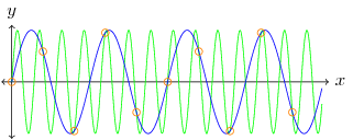
In order to sample this signal and prevent the loss of any information, the signal must be sampled at, or greater than, a rate twice the maximum bandwidth, . This is known as the Nyquist rate of the signal. If a signal is sampled at a frequency of , then any frequencies lower than may be aliased, that is, they may show up as artificial frequencies. This is known as the Nyquist frequency of the sampling system. Recall that , which produces a copy of the frequency response at every impulse, that is, at at spacing of in the frequency domain. When , then overlapping occurs between the copies of . The superposition principle tells us that the frequency response at these overlaps will be summed, introducing an artificial frequency response. Since the frequency domain representation is symmetric about the origin () the sampling frequency must be twice as large as in order to prevent any overlap. The green waveform in Figure 1 represents a frequency greater than that was aliased to a lower frequency. Figure 2 shows two sinusoids, if the signal is sampled at the orange points the two sinusoids are indistinguishable because the frequency of the green sinusoid is greater than the Nyquist rate.

Figure 2. Aliased Sinusoids

If the sampling is done at a rate greater than the Nyquist rate, then the no information is lost and the continuous-time signal can be fully reconstructed from the discrete-time signal. In order to reconstruct the continuous-time signal from the discrete-time signal we want to extract a copy of the frequency response and do an inverse Fourier transform. Remember that convolving with the impulse train created copies of the frequency response at each impulse. We only want one copy of the frequency response, so we want to multiply by a rectangular window with unit height on the interval and 0 everywhere else, referred to as the ideal reconstruction filter. This is equivalent to convolving the impulse response in the spatial domain with the spatial representation of the ideal reconstruction filter, referred to as the ideal sync, shown in Figure 3.

Figure 3. Ideal Sync

Read More

Stochastic Processes and Markov Chains

The term stochastic describes a system which has some element of randomness, and is therefore non-deterministic. A stochastic process is a process in which the transitions from one state to another may include some measure of uncertainty. Since there may be some uncertainty regarding state of the process at any given time it is natural to represent the state as a random variable. A stochastic process is modeled as a sequence of random variables representing the state indexed by a time variable, or .

A Markov chain is a type of stochastic process which exhibits the Markov property. That is, the future states of the process do not depend statistically on the past states. In terms of conditional probability (link):

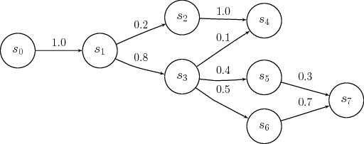
The probability of being in state at time is conditional only on the state at time and not on the previous states . Strictly speaking this is a first order Markov chain. The state at time of a chain of order, or memory, depends on the previous states. Figure 1 shows an example of a Markov chain.

Figure 1. Markov Chain
Figure 1. Example Markov Chain

We can define a variable to be the probability that the process transitions from state to state at time . This is called a single step transition probability. This idea can be extended to an n-step transition probability , that is, the probability that the process transitions from state to state in steps. The probability that the process in any particular state at time is given by the weighted sum of the transition probabilities for all states that the process could have been in at time . It can also be calculated as the sum of the -step transition probabilities starting at a time .

Since the probabilities of events in a sample space must sum to 1, we say that a vector who’s elements are non-negative real numbers and sum to 1 is a stochastic vector. Likewise a stochastic matrix may be defined depending on the meanings of the rows and columns. The usual meaning, and the one we will use here, is that each row of the matrix is a stochastic vector, called a right stochastic matrix. Given the transition probabilities from state to state it is natural to arrange these probabilities in a stochastic matrix. This matrix is called the transition matrix, , such that as defined above. The probability of transitioning from state to in steps is . For completeness the transition matrix , that is, when the transition matrix is the identity matrix.

The random variable representing the state of the process at time can be manipulated as a stochastic vector, where element is the probability that the process is in state . The initial state of the system can be given as a stochastic vector .

A state is said to be accessible from state , () if for some . If and then and are said to communicate (). A set of states which all communicate with each other and communicate with no other states forms an equivalence class called a communicating class. Furthermore, a communicating class can be closed if the probability of leaving the class is zero, . If the entire state space of a Markov chain is a communicating class than the chain is said to be irreducible. The graph of an irreducible Markov chain is a connected graph.

Cycles within the graph of the Markov chain lead to a notion of periodicity. A state has a period of if and is always a multiple of , that is, is the greatest common divisor of all possible . If then the state is called aperiodic. A Markov chain itself is said to be aperiodic if every state in the chain is aperiodic. If there is a non-zero probability of never returning to state from state then the state is said to be transient. A non-transient state is called recurrent or persistent.

In the special case that a Markov chain is both irreducible and aperiodic it is called ergodic, meaning that it converges to a single unique stationary distribution, called the equilibrium distribution, regardless of the initial distribution. A stationary distribution is a stochastic vector where each element satisfies the property:

Read More

Fourier Transforms

Usually when a signal is captured the domain is either temporal or spatial. For example, an audio signal from a microphone measures changes in air pressure (sound waves) over time, thus the measurements are in the time domain. An image sensor takes measurements from an array of photoreceptors, thus the signal exists in the spatial domain. A video signal is both in the time domain and the spatial domain. It can be helpful to deal with a signal in different domains, for example the frequency domain. Here the value of a signal at a given point represents the contribution to the signal from a sinusoid at a certain frequency. So instead of representing an amplitude at time , it represents the contribution to the signal by a sinusoid at frequency . The Fourier Transform transforms a signal into the frequency domain.

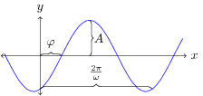
A sinusoid is any function that takes the form , where is the amplitude, is the angular frequency, and is the phase, as shown in Figure 1. The angular frequency is measured in radians per second, therefore is one full cycle, sometimes denoted for frequency, in cycles per second or hertz (Hz). One full cycle is called the period, .

Figure 1. Sinusoid
Figure 1. Sinusoid

Another way of representing a sinusoid is with a complex exponential, in the form . Euler’s formula tells us that this is equal to a complex number where the real part is and the imaginary part is . Just as we can represent a discrete-time signal as a linear combination (scaled, shifted) of unit impulses, a periodic discrete-time signal can be expressed as the linear combination of sinusoids. The Discrete-Time Fourier Transform, or DTFT, decomposes a discrete-time signal into the composite sinusoids. The sinusoids act as a basis set for the signal, in the same way that the and vectors form the basis set for 2-dimensional Cartesian space. The DTFT is given in the following equation:

In my previous article I mentioned that the discrete-time signal is derived from a continuous signal in the form , where is the sampling period. The inverse of the sampling period is the sampling frequency, which corresponds to the number of samples per second. Due to limitations of sampling a continuous signal, we often represent the frequencies in relation to the sampling frequency. This is called a normalized frequency, in terms of hertz it is the number of cycles per sample, equal to , or in terms of angular frequency it is the number of radians per sample, equal to . Since radians are a unit-less measurement the normalized angular frequency is sometimes referred to as inverse samples. For example, the following signal in Figure 2 can be decomposed into the sinusoids at the frequencies plotted in Figure 3; the sinusoids themselves are shown in Figure 4.

Figure 2. Example Signal Waveform
Figure 3. Frequency Domain
Figure 4. Composite Sinusoids

The Fourier series allows us to perform an inverse Fourier Transform to reconstruct a time-domain signal from the composite sinusoids using the complex exponential form:

Since the frequency domain representation is a sum of scaled complex exponentials, it is a complex function. The magnitude represents the amplitude of the sinusoid, while the angle or argument represents the phase.

Consider an LTI system with impulse response and output given inputs in the form of a complex exponentials:

In the last equation above, the function is called the frequency response of the system. We can see that is the Fourier transform of the impulse response . Also, instead of convolving the frequency response with the input, it is multiplied. In general we can relate the time-domain signals to their frequency domain representations as follows:

Read More

Introduction to Signal Processing

The term signal processing refers the manipulation of a signal or varying quantity. A signal is often a sequence of measurements taken by some sensor. The quantities may vary over time or space, or both. We represent a 1-dimensional signal as a continuous function, usually denoted . However, in digital signal processing we often want to deal with discrete-time signals, where the the signal function takes on values at discrete time steps. This is typically denoted where is the sample period, that is, the time between samples. A discrete-time system transforms a discrete-time signal onto a new unique discrete-time signal. We will represent this transformation with the operator such that .

For the purposes of this article we will be concerned with linear, time-invariant systems, or LTI systems. If a system is linear, it means that obeys the rule of superposition. The rule of superposition states that the net response at a given place and time caused by two or more stimuli is the sum of the responses of each stimulus individually1, that is:

A time-invariant, or shift-invariant, transform is one for which a shift in the input causes a similar shift in the output:

The output of linear time-invariant system can be fully characterized by a function of the input, called the impulse response. This is useful because the output of a system can be derived by simply convolving the input with the impulse response. This will be discussed in detail later in this post.

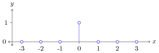
A discrete-time signal can be fully represented as a sum of scaled and shifted unit impulses. The unit impulse is a function representing the Kronecker Delta , shown in Figure 1. In general, a function can be represented as . The unit impulse will only be 1 when and will be scaled by .

Figure 1. Unit Pulse or Kronecker Delta Function
Figure 1. Unit Pulse or Kronecker Delta

Let us look at how the LTI transform behaves when we represent our input function as a sum of scaled unit pulses:

In the last step the function is the impulse response. You can see why it is named this since it is the system’s response to the unit impulse. The sum of scaled impulse responses is called the convolution sum. The convolution of two functions and is denoted with the convolution operator . So the output of an LTI system is the convolution of the input with the impulse response: . This amounts to the summation of the product of the two functions, one being reversed and shifted. Note that convolution is commutative, , so it does not matter which function is reversed and shifted. Convolution is also distributive over addition, , and associative, . Convolution can easily be extended to multi-dimensional functions. For example, the convolution sum for a 2-dimensional function is given as:

Often we know the input to the system and we wish to create an output with desired characteristics. In this case we wish the impulse response to act as a filter. Since the system is fully characterized by the impulse response, by expressing how we wish the system to respond to an impulse we can define how the whole system will respond to input in general.

Read More