One fundamental class of operations that can be performed to extract information from a signal is that of derivative operations. Just as derivatives are used in calculus to extract features of a curve or surface, the same ideas can be applied to a signal.
The first problem we have is that of taking the derivative of a discrete-time signal. Discrete-time signals are not continuous and are non-differentiable. However, we do know that if the Nyquist Rate was met when sampling, the continuous-time signal should be reconstructable from the discrete-time signal using the ideal sync. In order to reconstruct the continuous-time signal, the discrete-time signal is convolved with the ideal sync, . So if we want the derivative of the continuous time signal, we can start by taking the derivative of both sides of this equation.
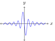
So the derivative of the continuous-time signal is equal to the convolution of the discrete-time signal with the derivative of the ideal sync. If instead the discrete-time signal is convolved with the sampled derivative ideal sync, this will result in a sampled derivative of the continuous-time signal, . The derivative of the ideal sync is shown in Figure 1. The major problem with this approach is that the derivative of the ideal sync is infinite and does not fall off rapidly.

Designing filters to approximate the discrete-time derivative of the ideal sync are beyond the scope of this article, but several popular techniques will be described later.
If we want to apply derivative operations to an image we will have to extend this idea into 2-dimensional space. Using partial differentiation and a 2-dimensional ideal sync results in the following derivatives for :
The 2-dimensional ideal sync is said to be separable since it can be separated into its 1-dimensional components, . Again, these continuous-time derivatives of the ideal sync must be sampled. The horizontal and vertical derivative filters are denoted and , respectively.
The most basic approach to approximating is to use a version of the difference operator, that is, a sum of scaled differences of the samples, such as . This is accomplished by convolving with and amounts to an approximation of the derivative. Figure 2 shows an example of a row of pixel values from an image, while Figure 3 shows the derivative approximation of the pixel values and Figure 4 shows the second derivative. The locations where the intensity values change the most rapidly are represented by local peaks in the first derivative and zero-crossings in the second derivative. Note that taking the derivative extends the range of intensity values to allow negative values.


If we think of the partial derivatives in each dimension as a component of a vector, this vector will represent the rate of change of the signal and the direction. This is called the gradient of the signal:
The gradient is a vector field where the direction of the vector at each point represents the direction of maximum change, while the magnitude of the vector represents the amount of change. As with other vectors, the magnitude can be calculated as , and the direction as . Given filters in the x and y directions, we can also construct a filter for an arbitrary direction, . Figure 4 shows a sample image and Figures 5 & 6 show the partial derivatives with respect to x and y respectively.
 |
 |
 |
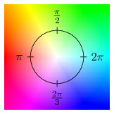
Figure 7 shows both the magnitude and the direction of the gradient of the sample image using the colormap in Figure 8. The partial derivative with respect to any direction, not just horizontal and vertical, can be calculated by multiplying a vector with the gradient, .
 |
 |
A useful tool when dealing with the second derivatives is the Hessian matrix which combines the derivatives into a matrix of the following form:
![]()
Where is the partial derivative of with respect to , i.e. the second derivative. To calculate the second derivative with respect to two vectors we can use the Hessian: .