Sampling Theory

This article will deal with sampling and reconstructing signals. Introductory information to signal processing can be found here, and background on Fourier Transforms can be found here. Sampling a continuous-time signal to a discrete-time signal involves measuring a series of data points on a continuous waveform. Ideally the discrete-time signal should contain all of the information of the continuous-time signal. If the sampling period is too small, it is possible to lose information when sampling. The act of sampling a continuous-time signal can be modeled by multiplying the signal by an impulse train, or Dirac comb. Similar to the discrete-time Kronecker delta, the Dirac delta function represents an impulse as a continuous function:

The impulse train is formed by taking a sum of shifted Dirac deltas, . Multiplying the signal with the impulse train gives a continuous-time signal with scaled impulses at frequency , called an ideal sampler, . The frequency domain representation of an impulse train is also an impulse train, with impulses at . In the frequency domain this corresponds to convolving the ideal sampler with the frequency representation of the signal, . Consider the frequency domain representation shown in Figure 1. The blue curve represents a signal which is called a bandlimited signal because it contains no energy at frequencies above a certain frequency, or bandwidth, .

Figure 1. Bandlimited Signal and Alias

In order to sample this signal and prevent the loss of any information, the signal must be sampled at, or greater than, a rate twice the maximum bandwidth, . This is known as the Nyquist rate of the signal. If a signal is sampled at a frequency of , then any frequencies lower than may be aliased, that is, they may show up as artificial frequencies. This is known as the Nyquist frequency of the sampling system. Recall that , which produces a copy of the frequency response at every impulse, that is, at at spacing of in the frequency domain. When , then overlapping occurs between the copies of . The superposition principle tells us that the frequency response at these overlaps will be summed, introducing an artificial frequency response. Since the frequency domain representation is symmetric about the origin () the sampling frequency must be twice as large as in order to prevent any overlap. The green waveform in Figure 1 represents a frequency greater than that was aliased to a lower frequency. Figure 2 shows two sinusoids, if the signal is sampled at the orange points the two sinusoids are indistinguishable because the frequency of the green sinusoid is greater than the Nyquist rate.
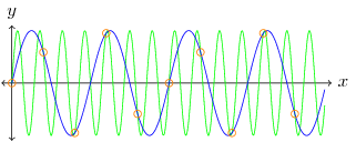
Figure 2. Aliased Sinusoids

If the sampling is done at a rate greater than the Nyquist rate, then the no information is lost and the continuous-time signal can be fully reconstructed from the discrete-time signal. In order to reconstruct the continuous-time signal from the discrete-time signal we want to extract a copy of the frequency response and do an inverse Fourier transform. Remember that convolving with the impulse train created copies of the frequency response at each impulse. We only want one copy of the frequency response, so we want to multiply by a rectangular window with unit height on the interval and 0 everywhere else, referred to as the ideal reconstruction filter. This is equivalent to convolving the impulse response in the spatial domain with the spatial representation of the ideal reconstruction filter, referred to as the ideal sync, shown in Figure 3.

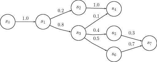
Figure 3. Ideal Sync

Read More

Stochastic Processes and Markov Chains

The term stochastic describes a system which has some element of randomness, and is therefore non-deterministic. A stochastic process is a process in which the transitions from one state to another may include some measure of uncertainty. Since there may be some uncertainty regarding state of the process at any given time it is natural to represent the state as a random variable. A stochastic process is modeled as a sequence of random variables representing the state indexed by a time variable, or .

A Markov chain is a type of stochastic process which exhibits the Markov property. That is, the future states of the process do not depend statistically on the past states. In terms of conditional probability (link):

The probability of being in state at time is conditional only on the state at time and not on the previous states . Strictly speaking this is a first order Markov chain. The state at time of a chain of order, or memory, depends on the previous states. Figure 1 shows an example of a Markov chain.

Figure 1. Markov Chain
Figure 1. Example Markov Chain

We can define a variable to be the probability that the process transitions from state to state at time . This is called a single step transition probability. This idea can be extended to an n-step transition probability , that is, the probability that the process transitions from state to state in steps. The probability that the process in any particular state at time is given by the weighted sum of the transition probabilities for all states that the process could have been in at time . It can also be calculated as the sum of the -step transition probabilities starting at a time .

Since the probabilities of events in a sample space must sum to 1, we say that a vector who’s elements are non-negative real numbers and sum to 1 is a stochastic vector. Likewise a stochastic matrix may be defined depending on the meanings of the rows and columns. The usual meaning, and the one we will use here, is that each row of the matrix is a stochastic vector, called a right stochastic matrix. Given the transition probabilities from state to state it is natural to arrange these probabilities in a stochastic matrix. This matrix is called the transition matrix, , such that as defined above. The probability of transitioning from state to in steps is . For completeness the transition matrix , that is, when the transition matrix is the identity matrix.

The random variable representing the state of the process at time can be manipulated as a stochastic vector, where element is the probability that the process is in state . The initial state of the system can be given as a stochastic vector .

A state is said to be accessible from state , () if for some . If and then and are said to communicate (). A set of states which all communicate with each other and communicate with no other states forms an equivalence class called a communicating class. Furthermore, a communicating class can be closed if the probability of leaving the class is zero, . If the entire state space of a Markov chain is a communicating class than the chain is said to be irreducible. The graph of an irreducible Markov chain is a connected graph.

Cycles within the graph of the Markov chain lead to a notion of periodicity. A state has a period of if and is always a multiple of , that is, is the greatest common divisor of all possible . If then the state is called aperiodic. A Markov chain itself is said to be aperiodic if every state in the chain is aperiodic. If there is a non-zero probability of never returning to state from state then the state is said to be transient. A non-transient state is called recurrent or persistent.

In the special case that a Markov chain is both irreducible and aperiodic it is called ergodic, meaning that it converges to a single unique stationary distribution, called the equilibrium distribution, regardless of the initial distribution. A stationary distribution is a stochastic vector where each element satisfies the property:

Read More

Fourier Transforms

Usually when a signal is captured the domain is either temporal or spatial. For example, an audio signal from a microphone measures changes in air pressure (sound waves) over time, thus the measurements are in the time domain. An image sensor takes measurements from an array of photoreceptors, thus the signal exists in the spatial domain. A video signal is both in the time domain and the spatial domain. It can be helpful to deal with a signal in different domains, for example the frequency domain. Here the value of a signal at a given point represents the contribution to the signal from a sinusoid at a certain frequency. So instead of representing an amplitude at time , it represents the contribution to the signal by a sinusoid at frequency . The Fourier Transform transforms a signal into the frequency domain.

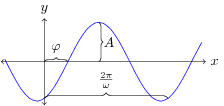
A sinusoid is any function that takes the form , where is the amplitude, is the angular frequency, and is the phase, as shown in Figure 1. The angular frequency is measured in radians per second, therefore is one full cycle, sometimes denoted for frequency, in cycles per second or hertz (Hz). One full cycle is called the period, .

Figure 1. Sinusoid
Figure 1. Sinusoid

Another way of representing a sinusoid is with a complex exponential, in the form . Euler’s formula tells us that this is equal to a complex number where the real part is and the imaginary part is . Just as we can represent a discrete-time signal as a linear combination (scaled, shifted) of unit impulses, a periodic discrete-time signal can be expressed as the linear combination of sinusoids. The Discrete-Time Fourier Transform, or DTFT, decomposes a discrete-time signal into the composite sinusoids. The sinusoids act as a basis set for the signal, in the same way that the and vectors form the basis set for 2-dimensional Cartesian space. The DTFT is given in the following equation:

In my previous article I mentioned that the discrete-time signal is derived from a continuous signal in the form , where is the sampling period. The inverse of the sampling period is the sampling frequency, which corresponds to the number of samples per second. Due to limitations of sampling a continuous signal, we often represent the frequencies in relation to the sampling frequency. This is called a normalized frequency, in terms of hertz it is the number of cycles per sample, equal to , or in terms of angular frequency it is the number of radians per sample, equal to . Since radians are a unit-less measurement the normalized angular frequency is sometimes referred to as inverse samples. For example, the following signal in Figure 2 can be decomposed into the sinusoids at the frequencies plotted in Figure 3; the sinusoids themselves are shown in Figure 4.

Figure 2. Example Signal Waveform
Figure 3. Frequency Domain
Figure 4. Composite Sinusoids

The Fourier series allows us to perform an inverse Fourier Transform to reconstruct a time-domain signal from the composite sinusoids using the complex exponential form:

Since the frequency domain representation is a sum of scaled complex exponentials, it is a complex function. The magnitude represents the amplitude of the sinusoid, while the angle or argument represents the phase.

Consider an LTI system with impulse response and output given inputs in the form of a complex exponentials:

In the last equation above, the function is called the frequency response of the system. We can see that is the Fourier transform of the impulse response . Also, instead of convolving the frequency response with the input, it is multiplied. In general we can relate the time-domain signals to their frequency domain representations as follows:

Read More

Introduction to Signal Processing

The term signal processing refers the manipulation of a signal or varying quantity. A signal is often a sequence of measurements taken by some sensor. The quantities may vary over time or space, or both. We represent a 1-dimensional signal as a continuous function, usually denoted . However, in digital signal processing we often want to deal with discrete-time signals, where the the signal function takes on values at discrete time steps. This is typically denoted where is the sample period, that is, the time between samples. A discrete-time system transforms a discrete-time signal onto a new unique discrete-time signal. We will represent this transformation with the operator such that .

For the purposes of this article we will be concerned with linear, time-invariant systems, or LTI systems. If a system is linear, it means that obeys the rule of superposition. The rule of superposition states that the net response at a given place and time caused by two or more stimuli is the sum of the responses of each stimulus individually1, that is:

A time-invariant, or shift-invariant, transform is one for which a shift in the input causes a similar shift in the output:

The output of linear time-invariant system can be fully characterized by a function of the input, called the impulse response. This is useful because the output of a system can be derived by simply convolving the input with the impulse response. This will be discussed in detail later in this post.

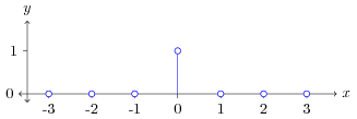
A discrete-time signal can be fully represented as a sum of scaled and shifted unit impulses. The unit impulse is a function representing the Kronecker Delta , shown in Figure 1. In general, a function can be represented as . The unit impulse will only be 1 when and will be scaled by .

Figure 1. Unit Pulse or Kronecker Delta Function
Figure 1. Unit Pulse or Kronecker Delta

Let us look at how the LTI transform behaves when we represent our input function as a sum of scaled unit pulses:

In the last step the function is the impulse response. You can see why it is named this since it is the system’s response to the unit impulse. The sum of scaled impulse responses is called the convolution sum. The convolution of two functions and is denoted with the convolution operator . So the output of an LTI system is the convolution of the input with the impulse response: . This amounts to the summation of the product of the two functions, one being reversed and shifted. Note that convolution is commutative, , so it does not matter which function is reversed and shifted. Convolution is also distributive over addition, , and associative, . Convolution can easily be extended to multi-dimensional functions. For example, the convolution sum for a 2-dimensional function is given as:

Often we know the input to the system and we wish to create an output with desired characteristics. In this case we wish the impulse response to act as a filter. Since the system is fully characterized by the impulse response, by expressing how we wish the system to respond to an impulse we can define how the whole system will respond to input in general.

Read More