Like any captured signal, photographic images often suffer from the presence of noise. Noise produces variations in the captured signal that do not occur in the natural signal. That is, noise is introduced somewhere in the process of capturing the signal. It is usually viewed as an unwanted corruption of the signal, therefore the modeling and elimination of noise is an important part of signal processing. Noise can occur in a pattern, or be complex enough that it is modeled as a random phenomenon.
Noise can have many difference causes, and therefore manifest itself in many different ways. “Salt and pepper” noise is the term given to noise which causes the value of the signal at a particular point to be a random value. This has the effect of causing random spikes in the captured signal, regardless of the original signal, often called impulse noise. Quantizing the signal may cause noise as it is effectively assigning a particular value to a range of possible values, and therefore modifying the original values in a certain pattern. A common type of noise in amplified signals is Gaussian noise. The noise factor can be thought of as a random variable that follows a normal, or Gaussian, distribution. The noise factor can be added to the pixel value, called additive noise, or multiplied with the pixel value, multiplicative noise. When dealing with a potentially noisy signal it is often sufficient to take Gaussian noise into account to get acceptable results. Gaussian noise occurs in digital imagery as fluctuations in intensity values of the image. The noise is pixel-independent, meaning that the change in a pixel value is independent of the change in any other pixel value. It is also independent of the original intensity at each pixel. Since Gaussian noise is common and relatively simple it is commonly taken into consideration in generalized signal processing methods.
Noise can contribute noticeable artificial components to the image signal. Smoothing or blurring is a type of operation which attempts to eliminate the noise while preserving the structure of the image. The primary way this is accomplished is through the use of neighborhood filters. These are kernels, or matrices, which are convolved with the image in order to achieve some transformation, in this case smoothing.
One assumption we may be able to make is that the value of a pixel is relatively similar to the value of the neighboring pixels. Therefore, averaging together the pixel values in a small neighborhood should preserve the structure of the image while attenuating the effects of outlier values (the noise). This methods is called average smoothing, and is accomplished by convolving the image with a kernel in the following form, called a box filter:

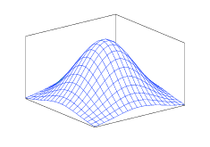
One issue with the box filter is that its rectangular window produces undesirable effects in the frequency domain. A Gaussian smoothing kernel provides a much better approximation of ideal smoothing. Intuitively the idea is that the neighboring pixels which are closer to the target pixel are weighted more heavily in the average than the pixels farther away. The weight coefficients follow a Gaussian distribution, producing a filter like the one shown in Figure 1. The Gaussian filter is desirable because of its gradual cutoff, producing a Gaussian distribution in the frequency domain as well which delivers smooth monotonically decreasing attenuation of higher frequencies. A Gaussian distribution has infinite width, however, the tails approach zero relatively rapidly so a few standard deviations of width are sufficient for accurate results.
![]()

Figure 2 shows a sample image and Figures 3, 4, & 5 show the effects of successively larger Gaussian smoothing kernels.
| Â Â
Â
|
 Â
Â
|
 Â
Â
|
 Â
Â
|


