The term signal processing refers the manipulation of a signal or varying quantity. A signal is often a sequence of measurements taken by some sensor. The quantities may vary over time or space, or both. We represent a 1-dimensional signal as a continuous function, usually denoted . However, in digital signal processing we often want to deal with discrete-time signals, where the the signal function takes on values at discrete time steps. This is typically denoted where is the sample period, that is, the time between samples. A discrete-time system transforms a discrete-time signal onto a new unique discrete-time signal. We will represent this transformation with the operator such that .
For the purposes of this article we will be concerned with linear, time-invariant systems, or LTI systems. If a system is linear, it means that obeys the rule of superposition. The rule of superposition states that the net response at a given place and time caused by two or more stimuli is the sum of the responses of each stimulus individually1, that is:
A time-invariant, or shift-invariant, transform is one for which a shift in the input causes a similar shift in the output:
The output of linear time-invariant system can be fully characterized by a function of the input, called the impulse response. This is useful because the output of a system can be derived by simply convolving the input with the impulse response. This will be discussed in detail later in this post.
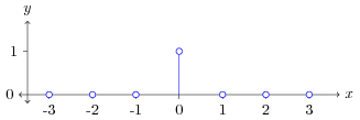
A discrete-time signal can be fully represented as a sum of scaled and shifted unit impulses. The unit impulse is a function representing the Kronecker Delta , shown in Figure 1. In general, a function can be represented as . The unit impulse will only be 1 when and will be scaled by .

Let us look at how the LTI transform behaves when we represent our input function as a sum of scaled unit pulses:
In the last step the function is the impulse response. You can see why it is named this since it is the system’s response to the unit impulse. The sum of scaled impulse responses is called the convolution sum. The convolution of two functions and is denoted with the convolution operator . So the output of an LTI system is the convolution of the input with the impulse response: . This amounts to the summation of the product of the two functions, one being reversed and shifted. Note that convolution is commutative, , so it does not matter which function is reversed and shifted. Convolution is also distributive over addition, , and associative, . Convolution can easily be extended to multi-dimensional functions. For example, the convolution sum for a 2-dimensional function is given as:
Often we know the input to the system and we wish to create an output with desired characteristics. In this case we wish the impulse response to act as a filter. Since the system is fully characterized by the impulse response, by expressing how we wish the system to respond to an impulse we can define how the whole system will respond to input in general.
2 thoughts on “Introduction to Signal Processing”
Comments are closed.