See my previous post on random variables for more background. This post will cover a few important statistical measures that help characterize the probability distribution of a random variable and the relationship between random variables. The first is the expected value or mean is denoted or for random variable . For a discrete random variable the expected value equates to a probability-weighted sum of the possible values of the variable, . The sample mean, , is the average of a collected sample, that is the sum of the values, divided by the number of values. The law of large numbers states that the sample mean approaches the expected value in the limit of the number of samples collected. Note that the expected value may not be an actual value that the random variable may take on. For example, the expected value of a random variable that represents the roll of a die is
The expected value function is linear, meaning that the following property holds:
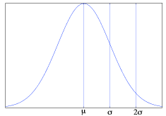
Variance is a measure that typically describes how “spread out” a distribution is. It is denoted , or , and is defined as the expected value of the difference between the random variable and the mean of the distribution squared, . It can also be defined as the difference between the expected value of the random variable squared and the squared expected value of the variable, . If you have a sample the variance can be defined as the scaled sum of the differences between the samples and the mean for samples. The square root of the variance is called the standard deviation and is commonly used as well. Figure 1 shows the relationship between expected value and variance on a normal distribution.

The law of large numbers states that as the number of observations of a random variable increases, the mean of the sample converges toward the expected value of the random variable. When making observations of a large number of independent and identically distributed random variables, the central limit theorem claims that as the number of random variables increases, the sample means of the random variables will fall into an approximately normal distribution. This normal distribution will have the same expected value as the distribution of the random variables, and a variance of , where is the finite variance of the random variable distribution and is the number of random variables.
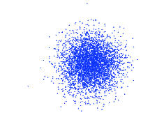
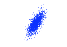
When looking at the relationship between two random variables, it is often useful to see how they change with respect to their expected values. Covariance is a measure of the correlation between two variables. For example, if one variable tends to be above its mean when the other is above as well, then their covariance is positive, while if one tends to be below its mean when the other is above their covariance is negative. Covariance is defined as or . When covariance is normalized, it is called the correlation, given by the following formula: . Figures 2 and 3 illustrate how covariance and correlation represent the relationship between variables. In Figure 2 the two random variables are characterized by independent normal distributions. Their covariance and correlation are both around ~0.01. In Figure 3 the second random variable is a copy of the first random variable with a small amount of Gaussian noise added.


One thought on “Statistical Metrics”
Comments are closed.